Executive Methods for Problem Solution: 2018-02-04

Friday, February 9, 2018

A Model to Solve a System of Nonlinear Equations by Using Microsoft Excel

This is an example for solving a system of nonlinear equations by using the Big Data Science Analysis with Microsoft excel plus VBA.

Definitely, there are many complicated problems that can be solved by using this analytic model. For instance, one of the applications of this model is to solve problems related to optimization, such as Hill Climbing.

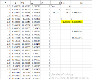
For example, what is the maximum area of a rectangle inscribed in a circle with a radius of 2 units?

You can find the answers for “x” and “y” in this rectangle in the below data analysis:

I would like to inform you that this model is able to solve all linear and nonlinear system of equations in which it gives us less error than traditional methods such as Newton – Raphson , Gauss – Seidel, Jacobian and so on. Don't worry, if you have not any knowledge about traditional methods. Dive into new technology.

Example: A Model to Track the Location of a Particle in the Space

One of the most important needs for many projects is, quickly to track the motion of a particle when

it is tripping between two points in the space. For instance, suppose particle P is moving by velocity “V” with accelerate equal to zero from point A (x1, y1, z1) to point B (x2, y2, z2). We want to know the coordination of P (x, y, z) at the moment of “t” when it is moving in direction of A to B. This model gives us the opportunity to obtain the coordination P (x, y, z) only by click. In fact, if we have the coordination P (x, y, z), it will be as an index for us that other particles which are moving from A to B such as P1, P2, …. are not tripping in the exact direction of A to B. In this case, we have to solve a system of two nonlinear equations as follows:

First of all, we should define amount of “a” and “b” as follows:

The distance of point A to point B is calculated by using below formula and also “X” is the distance that particle P will travel after time “t” in direction of A to B:

Therefore, we should solve below system of two nonlinear equations

Below figure as well as shows you the components of this model

Let me explain you about the components of above model as follows:

1. In right side on cells G4:J10, we have inputs including the coordination points A and B, velocity of particle P (v), the time after staring to travel particle P (t) and Error which is the difference between the results. So, X = v.t, d = distance between point A and B and on cell G10, I have included a logic formula (=if (H8 >= H9, H8, 0)). It means, if X = 0 then the particle has passed point B

2. In left side on cells C5:E6, we have other inputs including the ranges to reach to the answer for coordination particle P (x, y, z) which is the solution for system of two nonlinear equations.
Here, there are lower and upper ranges which are changed by click on cell A2 and also this change will again go back by click on cell B2 (Go & Back).

This part has been utilized by the method stated in article of “Can We Solve a Nonlinear Equation with Many Variables?” posted on link:
http://emfps.org/2016/10/can-we-solve-nonlinear-equation-with.html

3. On cells C9:E9, we have outputs which are the answer to above

system of two nonlinear equations.

4. On cells C12:E13, we have Control (1) where first equation is solved by using the coordination A

and P and it is compared with amount of “X^2” on cell C14. So, second equation is solved by using the coordination B and P and it is also compared with amount of “(d-X)^2”on cell C15. The differences have been mentioned on cell G12 and G13 as the errors.

5. On cells E15:G17, we have Control (2) which is referred to track the directions in which we are willing to know if the motion of particle P is in direction from point A to point B. In this case, a control can be conducted by using below formulas:

You can see below screenshot as the examples for this model:

Conclusion

.Above article gives you a simple example

In fact, I am willing to tell you that this model is able to solve all system of two or three nonlinear

equations.

All researchers and individual people, who are interested in having this model, don’t hesitate to send
their request to below addresses:

https://t.me/Allisnumber

Monday, February 5, 2018

The Impact of Stochastic Matrix on Any Vector

A stochastic matrix shows us that the sum all elements on each column (or each row) is equal one or we can say that each column (or each row) of a stochastic matrix is just a probability vector.

Theorem (1): The sequence of operations a stochastic matrix on any vector will be finally obtained the constant vector. (The elements of vector are the members of Real Number)

V1 = V0 * M^1 , V2 = V1*M^2, V3 = V2*M^3, …. Vn+1 = V n* M^k

Where vector Vn+1 always will be the constant.

A special state is when the vector is a probability vector which is named Markov Chain or Markov Process

Example (1):

The sample of our vector (1*4) is:

V0 =

Suppose we have below stochastic matrix M (4*4):

M =

The results of the sequences (V0 * M) are as follows:

As we can see, the vectors of V5 and V6 are approximately the same.

Example (2):

The sample of our vector (1*4) is:

V0 =

The results of the sequences are as follows:

As we can see, the vectors of V5 and V6 are approximately the same.

An example for Markov Chain:

The sample of our probability vector (1*4) is:

V0 =

I consider above stochastic matrix M (4*4).

Then, we will have below results:

As we can see, the vectors of V5 and V6 are approximately the same.

Is below conjecture is a theorem?

Conjecture (1): The sequence of operations for transpose of a stochastic matrix (n*n) with non - zero elements on any vector will be finally obtained a vector with the same elements. (The elements of vector are the members of Real Number)