A Specific Permutation And Applications (1)

The base of the probability theory is always referred to permutations and combinations in which a permutation is an ordered combination. It means, if we have “n” events and choose “r” of them, we will have the opportunity to make many groups and subsets which are “r” from “n” where the repetition and the replacement will also give us new concepts.

As you know, basically we have two types of permutations:

1.      Permutations with repetition which is calculated by below formula:

The number of Permutations = n^r

2.      Permutations without repetition which is obtained by below formula:

            The number of Permutations = n!/(n-r)!

The purpose of this article is to introduce a specific permutation.

A specific permutation

Suppose we have a number of events “n” and we consider whole events as the pairs just like below set:

S = {(a1,a2), (b1,b2), (c1,c2), (d1,d2)….}

Here "S" is our sample space.
We are willing to make all permutations without repetition with “r” members from “S” where each set of permutations is included only one of the pairs. This is additional restriction for these permutations. It is clear; “r” must be always smaller or equal half of “n”.

Therefore, the characteristics of this specific permutation are defined as follows:

·        n = 2k   and   k ε N

·        r ≤ n/2

·        Each set of permutations is included only one of the pairs

The question is:  How can we calculate the number of these permutations?

By using below formula, we will be able to get the number of all permutations:

For instance, when we choose three choices from six events, we will have 48 permutations or if we have three choices from eight events, we will get 192 permutations.

By using Microsoft excel, we can generate all permutations on a spreadsheet of excel.

Example: Generating the Points on a Sphere

Suppose our sample space or events are pairs of plus and minus as follows:

S = {(-a, a), (-b, b), (-c, c)…}

In this case, for n = 6 we will have: 48 points which have been located on a sphere.

Assume we have the point P (2, 5, 24) in the 3D space in which the sample space will be below cited:

S = {(-2, 2), (-5, 5), (-24, 24)}

All below points are located on a sphere or gives us a field in 3D space:

Below model gives us all 48 points on a sphere when we have only coordination of one point:

In above model, the inputs are the coordination of one point P (x,y,z) and the outputs are the coordination of all 48 points on a sphere. As you can see, the radius of sphere (r) always stays the constant.

In the reference with above mentioned, below movie as well as shows an overall shape of this system when the location of a point is changed:

Does this conjecture lead us toward an absolute justice in the world?

Eigenvalue equal to the sum of all elements on each column or row

One of the properties two ways matrices which can be easily proved is, to obtain the Eigenvalue where the sum of all elements on each column or row is equal to Eigenvalue of these matrices.

Another interesting property of a two way matrix is, to have a special eigenvector that all elements of it are the same. It means, if “M” is a two ways matrix, vector “V” will be eigenvector of matrix “M” where we have:

V = (x, x, x, x, ….)  and    λ = the sum of all elements on each column or row

This property can be easily proved. 

Following to article of “The Impact of Stochastic Matrix on Any Vector”, let me tell you about another conjecture as follows:

Conjecture (2): The final result of Markov Process including the impact of a two ways stochastic matrix on any vector will be a vector with the same elements where each element will be equal to average all elements of initial vector.

Initial Vector: V0 = (a, b, c, d,….) and M = two ways stochastic matrix

Example:

Does this conjecture lead us toward an absolute justice in the world?

A Model for Analysis of Work Done by a Special Force

This model is an example as application one of theorems mentioned in article of “The Change Depends on the Direction of the Motion: The Symmetric Group Action (2)” posted on link:

http://www.emfps.org/2017/08/the-change-depends-on-direction-of_9.html?m=1

Work Done by Force

When we are speaking about the work done by a force, we have usually two options:

1. The work done on a particle by a constant force in magnitude and direction which is calculated by below equation:

2. The work done on a particle by a varying force in magnitude and direction in which we should use the line integral to calculate it as follows:

But, in this article, I am willing to introduce you a special force which has the constant magnitude but varying in direction. In this case, I have made a model that it is able to show us the location of the particle after being displaced by this special force.

Suppose a particle P (0, 0, 0) just like below figure being displaced by a force F:

Theorem: The force with below vector has the constant magnitude equal to 1.22474487139159 but varying in direction:

In this case, we can still use option (1) and below equation to calculate the work done:

Below figure shows the components of this model:

Let me explain you about the components of above model as follows:

1. In left side on cells C2:D3, we have inputs including the angle φ (degree) of force vector and amount of displacement of particle “P” which is “r”.

2. In right side on cells F3:J8, we have outputs including:

   2-1) on cells G3:I3, a special force vector can be calculated by using above theorem.

   2-2) on cells G4:I4, the direction of special force can be obtained by using below formula:

The magnitude of this force is the constant and equal to 1.22474487139159.

 2-3) on cell G5, we have the work done which is calculated by below formulas:

  2-4) on cells G7:I7, we have the location particle P (x, y, z) which is derived by this model.

  2-5) on cells G8:I8, the direction of motion particle P can be calculated by using below formula:

 2-6) The change of direction particle P will be done by click on cell A1 and also this change will again go back by click on cell B1 (Go & Back).  

You can see below screenshot as the examples for this model:

All researchers and individual people, who are interested in having this model, don’t hesitate to send their request to below addresses:

https://t.me/Allisnumber

A Model to Solve a System of Nonlinear Equations by Using Microsoft Excel

This is an example for solving a system of nonlinear equations by using the Big Data Science Analysis with Microsoft excel plus VBA.

Definitely, there are many complicated problems that can be solved by using this analytic model. For instance, one of the applications of this model is to solve problems related to optimization, such as Hill Climbing.

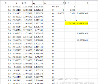
For example, what is the maximum area of a rectangle inscribed in a circle with a radius of 2 units?

You can find the answers for “x” and “y” in this rectangle in the below data analysis:

I would like to inform you that this model is able to solve all linear and nonlinear system of equations in which it gives us less error than traditional methods such as Newton – Raphson , Gauss – Seidel, Jacobian and so on. Don't worry, if you have not any knowledge about traditional methods. Dive into new technology.

Example: A Model to Track the Location of a Particle in the Space

 One of the most important needs for many projects is, quickly to track the motion of a particle when

it is tripping between two points in the space. For instance, suppose particle P is moving by velocity “V” with accelerate equal to zero from point A (x1, y1, z1) to point B (x2, y2, z2). We want to know the coordination of P (x, y, z) at the moment of “t” when it is moving in direction of A to B. This model gives us the opportunity to obtain the coordination P (x, y, z) only by click. In fact, if we have the coordination P (x, y, z), it will be as an index for us that other particles which are moving from A to B such as P1, P2, …. are not tripping in the exact direction of A to B. In this case, we have to solve a system of two nonlinear equations as follows:

 First of all, we should define amount of “a” and “b” as follows:

The distance of point A to point B is calculated by using below formula and also “X” is the distance that particle P will travel after time “t” in direction of A to B:

Therefore, we should solve below system of two nonlinear equations

Below figure as well as shows you the components of this model

Let me explain you about the components of above model as follows:

1. In right side on cells G4:J10, we have inputs including the coordination points A and B, velocity of particle P (v), the time after staring to travel particle P (t) and Error which is the difference between the results. So, X = v.t, d = distance between point A and B and on cell G10, I have included a logic formula (=if (H8 >= H9, H8, 0)). It means, if X = 0 then the particle has passed point B

2. In left side on cells C5:E6, we have other inputs including the ranges to reach to the answer for coordination particle P (x, y, z) which is the solution for system of two nonlinear equations. 
 Here, there are lower and upper ranges which are changed by click on cell A2 and also this change will again go back by click on cell B2 (Go & Back).

This part has been utilized by the method stated in article of “Can We Solve a Nonlinear Equation with Many Variables?” posted on link:
http://emfps.org/2016/10/can-we-solve-nonlinear-equation-with.html 

3. On cells C9:E9, we have outputs which are the answer to above 

system of two nonlinear equations.

4. On cells C12:E13, we have Control (1) where first equation is solved by using the coordination A 

and P and it is compared with amount of “X^2” on cell C14. So, second equation is solved by using the coordination B and P and it is also compared with amount of “(d-X)^2”on cell C15. The differences have been mentioned on cell G12 and G13 as the errors.

5. On cells E15:G17, we have Control (2) which is referred to track the directions in which we are willing to know if the motion of particle P is in direction from point A to point B. In this case, a control can be conducted by using below formulas:

You can see below screenshot as the examples for this model:

Conclusion

.Above article gives you a simple example

In fact, I am willing to tell you that this model is able to solve all system of two or three nonlinear   

equations.

All researchers and individual people, who are interested in having this model, don’t hesitate to send 
their request to below addresses:

https://t.me/Allisnumber

The Impact of Stochastic Matrix on Any Vector

A stochastic matrix shows us that the sum all elements on each column (or each row) is equal one or we can say that each column (or each row) of a stochastic matrix is just a probability vector.

Theorem (1): The sequence of operations a stochastic matrix on any vector will be finally obtained the constant vector. (The elements of vector are the members of Real Number)

V1 = V0 * M^1 , V2 = V1*M^2,  V3 = V2*M^3, …. Vn+1 = V n* M^k

Where vector Vn+1 always will be the constant.

A special state is when the vector is a probability vector which is named Markov Chain or Markov Process

Example (1):

The sample of our vector (1*4) is:

V0 =

                                                                        

Suppose we have below stochastic matrix M (4*4):

M =

The results of the sequences (V0 * M) are as follows:

As we can see, the vectors of V5 and V6 are approximately the same.

Example (2):

The sample of our vector (1*4) is:

V0 = 

The results of the sequences are as follows:

As we can see, the vectors of V5 and V6 are approximately the same.

An example for Markov Chain:

The sample of our probability vector (1*4) is:

V0 = 

I consider above stochastic matrix M (4*4).

Then, we will have below results:

As we can see, the vectors of V5 and V6 are approximately the same.

Is below conjecture is a theorem?

Conjecture (1): The sequence of operations for transpose of a stochastic matrix (n*n) with non - zero elements on any vector will be finally obtained a vector with the same elements. (The elements of vector are the members of Real Number)

Example (1):

Consider above stochastic matrix M (4*4):

M =

The transpose of matrix M is:

^MT =

The sample of vector is:

V0 = 

The results of the sequences are as follows:

As we can see, the elements of vector V7 are the same.

Example (2):

The sample of vector is:

V0 =

The results of the sequences are as follows:

As we can see, the elements of vector V7 are the same.