Powered By Blogger

Tuesday, August 16, 2016

The Calculation of Royalty Rate

Are you an engineer? What do you think about the value of your job? How can we get the value of engineering in a company? Or how can we calculate Intellectual property or royalty rate of a company?
To analyze some financial cases, we have to calculate the intellectual property of the company in additional to look at the book value on balance sheet.

Please see the case of "Yeats Valves and Controls Inc.". The end of first page of this case, Porter said: "YVC's prospects are brighter than ever. You have technology to die for. With our intellectual property and new products coming along, there is a lot of hidden value in this company that's not 
reflected on the balance sheet. Be a realist about the value"  

There are many papers and references to measure the intellectual property of a company. In this article, I chose a very fascinating hand book which presents six different methods to price the intellectual property of early-stage technologies.
The reference is as follows:

"ipHandbook of Best Practices"

Chapter 9.3 (2007) titled: "Pricing the Intellectual Property of Early-Stage
of Basic Valuation Technologies: A Primer Tools and Considerations" by RICHARD    RAZGAITIS

Posted on below link:


Even though I can say to you that above reference is very useful and interesting materials, there are some mistakes taken on method of Discounted Cash-Flow Analysis (method IV) and Table 14. For instance, when you read this method, you cannot still calculate the royalty rate. Your big question is: How has the royalty rate (12.6%) been calculated?

The purpose of my article is to improve and to explain the true method of Discounted Cash-Flow Analysis for calculating the royalty rate.

What should the items be improved?

1. Mistakes on calculations
2. The lack of enough information
3. The lack of good explanations

Let me start by the mistakes on calculations:
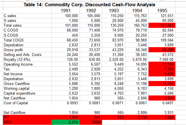
Here is Table 14:


As you can see, the calculation of all present values and total sales in 1995 are wrong. I corrected them on below spread sheet (Red highlights are true values):


2. The lack of enough information

When you start a discounted cash flow analysis, you should consider a terminal value for the end of your period. Because you have not the infinity cash in or cash out. Therefore, you should terminate and close your analysis by evaluating the value of your business in the end of the period. The formula for calculating Terminal value is as follows:

Terminal Value =
Free cash flow in the end of period * (1- terminal growth rate %) / (Cost of Capital % - terminal growth rate %)

For this analysis, I consider 2% for terminal growth rate. Please see my calculation of terminal value and also NPV on below spread sheet:


3. The lack of good explanations

The most important part of this article is, to calculate the royalty rate. The above reference do not show us how we can get the royalty rate equal to 12.6%.
Let me tell you the method as follows:

- At the first, you should eliminate amounts of Specialty product sales, Cost of specialty product sales and Royalty payment at 12.6% on your spread sheet and then calculate NPV just like below cited (Yellow highlights):


- In final step, you should add above amounts again and apply the sensitivity analysis for the royal rate and NPV in which NPV in both step are the same, it shows you percentage of the royalty rate as follows:


As you can see, the royalty rate is not 12.6% but it is equal to 55%.

Monday, August 1, 2016

A Template for Financial Section of a Business Plan Plus Monte Carlo Analysis

The most important part of a business plan is to prepare the financial section and the most crucial part of the financial section is, to predict assumptions because you should prove that your business plan is feasible or not.
The purpose of this article is to make a template of financial section on excel spreadsheets in which all excel files are connected together and also assumptions. In this case, you will be able to track 
rapidly your analysis by changing the assumptions.

Good news is to apply Monte Carlo analysis on this template in which you can control the risks of the assumptions and see the impact of them on your performance by using the method mentioned in below article: 


"Discounted Cash Flow Analysis plus Monte Carlo Method to Analyze Share Price of a Company" 
A sample for financial section of a business plan in service industry has been practiced on this 
template.

Financial Section of a Business Plan

A financial section of business plan is started by the assumptions. You can always change your assumptions and show to your client that this business plan is feasible or vice versa. Therefore, the assumptions play the most important role in your business plan. Traditionally, the people forecast the assumptions derived from financial data previous years of company or economic indicators. Definitely this method is not true due to high speed changes in the world. We have not still an accurate method to find out true assumptions. In fact, if we had a precise model to guess the assumptions, we could anticipate some share prices or the performances in stock markets. As I stated in my article of "External Real Forces and Pseudo-Forces to Design a Strategic Plan: Fuzzy logic Vs. Classic Logic" posted on link: http://emfps.blogspot.com/2013/12/external-real-forces-and-pseudo-forces.html, maybe the mathematics will give us an optimized model to forecast the 
assumptions in the near future.

What are the assumptions? They can be as follows:

- Initial investment
- The growth rate of the sales per year
-The growth rate of variable costs per year (COGS)
- The growth rate of fixed costs per year
- Terminal value growth rate
- The cost of capital (discounted rate) in each year
- Taxes
-Interest rates

When we obtain the assumptions, we should develop a cash flow statement for 12 months per year and predict it for 3 or 5 years in accordance with our initial investment and costs budgeting and also our assumptions. This is the statement that shows the money how is moving in and out of our business. Making a cash flow statement is very important for our business plan because it is the basic of profit – loss projection, balance sheet and finally our analysis.
After developing a cash flow statement, we will be able to prepare an Income statement projection (3 or 5 years) and by using data generated in profit – loss statement, we can make the Balance sheet projection for 3 or 5 years.
When we finish to create the cash flow statement, Income statement and Balance sheet, we will be ready to go our analytic process included in below steps:

- To calculate Key Ratios (Viability analysis) by using of Income statement and Balance sheet
- Break – Even Analysis by using of the Sales, Variable costs and Fixed costs
- Discounted Cash Flow Analysis
In my opinion, the most important part of our analytic process is, to go to the discounted cash flow analysis which is included three below steps:
- Pay Back analysis
- IRR analysis
- NPV analysis

Finally, we will have six excel files connected together and our assumptions as financial section of 
our business plan as follows:

- Cash flow statement
- Income statement
- Balance sheet
- Key Ratios (Viability analysis)
- Break – Even Analysis
- Discounted Cash Flow Analysis


A Sample of Financial Section for Business Plan in Service Industry

I have made a sample of a financial section for a business plan in the tourism industry. You can practice and also utilize this sample for commercial purposes. This sample can be used for many service industries, such as food service, boarding houses, restaurants, transportation, and so on
Firstly, we have assumptions as follows:


Then we develop a cash flow statement:


After that, we prepare an Income statement projection:


According to above mentioned, we can make Balance sheet:


Now, we can start the discount cash flow analysis as follows:


Then, we use from Pay back method:


Next analysis is, IRR and NPV method:


In this case, if we change some variables of our assumptions, we can see that all discounted cash flow analysis simultaneously change so that our business plan will not be feasible:


In fact, this is a goal for our analysis. In the near future, I will show you, how we can use from this method to reach the optimized variables? For instance, how can we obtain the bottom line for unit price of the goods?
Finally, we have Key ratios and Break – Even Analysis as follows:


Sunday, July 3, 2016

Model Predictive Control by Using Excel


Model Predictive Control (MPC) is a tool to control a system with multiple inputs and outputs. Nowadays, many researchers, managers and engineers are applying this tool in different fields such as financial management, strategic management and also many engineering fields.
Here I found two good links on Internet which give us some interesting examples and simulation 
models useful for piping engineers as follows:
 Model Predictive Control: Title
Video.icon.png Video lecture available for this section!  Note:
Bradley Anderson, Aaron Bennick, Michael Salciccioli: Authors
 sSarah Hebert, Valerie Lee, Matthew Morabito, Jamie Polan
Date Presented: 11/7/06; Revised: 10/30/07
Implementing MPC using Excel
In MPC, values of the control variables will be optimized for a given time interval in order to best tell the system how it should act. The control variables will be optimized by optimizing some characteristic. Usually, this characteristic is simply the least squared error between an actual state and a "set" or desired state. This can easily be done using the Solver tool in Excel.
You can find a good example of MPC and download excel spreadsheet for more practice on the above link.
Simulation of a Model Predictive Controller
You can also find an example on below link which gives us an application to simulate a Model Predictive Controller (MPC) for a single input, single output (SISO) first order with time delay process. You can download excel spread sheet for more practice.

Of course, always the assumptions and arrangement of components model have very important role to reach good predictions and valid results.  

Tuesday, June 28, 2016

The change depends on direction of the motion: Generating Eigenvalues from special matrices


"The change depends on direction of the motion"

This means: "It is possible, we move but there will not be any change or even we maybe lose everything."
"The change depends on direction of the motion." is a philosophic quote in which mathematics (Differential Calculus) applied it to find out the definition of gradient vector field.
For example, in Economics, USD is still an independent variable where many curves such as x = f ($), y = f ($), z = ($) … are determining the direction of motion overall function of
w = f (x, y, z …).
In designing strategic plan, maybe whole a company's strategy – making hierarchy depends on only a person or a department where this independent variable will change the company to a star or overturned (collapsed). In physics, the internal energy of the gas (except an ideal gas) depends on the pressure, volume and temperature (K = f (p, v, T)).
Nowadays, we can see many matrices as transformations and operators which are affecting on vectors.
The purpose of this article is, to introduce some special matrices in which you can easily generate all eigenvalues without any calculation.
The question is: How can we apply these special matrices as operators in our real world?


Some special matrices

1. Let consider “A1” as set of Arithmetic Progression where:

d = 1,      a1 = 1   and    an = a1 + (n - 1) d, n = 1, 2, 3,…..

In this case, we have:


A1 = {a1, (a1+1), (a2 +1),……. (a1 + (n - 1) d)}


One of permutations of set A1 is to invert members of set A1 as follows:


A2 = {(a1 + (n - 1) d),….,(a2 +1), (a1+1), a1}      

We can generate many sets which are the periodicity of set A1 just like below cited:

A3 = {a1, (a1+1), (a2 +1),……. (a1 + (n - 1) d)}

A4 = {(a1 + (n - 1) d),….,(a2 +1), (a1+1), a1}

Finally, we will have set B:

B = {A1, A2, A3, A4, …….An    


Rule 1: If size members of set Aor AorAor An, is equal to size members of set B, we will have a square matrix (Mn*n) to be generated by sets A1, A2, A3,…….An in which Eigenvalue of this matrix will be calculated by using of Binomial Coefficient as follows:

Eigenvalue (Mn*n) = Î» = C (k, 2)

Where:   k = n+1, nϵ N, Î» > 0


Example:
A1 = {1, 2, 3, 4}
A2 = {4, 3, 2, 1}      


A3 = {1, 2, 3, 4}

A4 = {4, 3, 2, 1}  


Matrix (M 4*4) = 
   
1 2 3 4

4 3 2 1

1 2 3 4

4 3 2 1

λ = C ((4+1), 2) = 10


2. Let consider set “A” as follows:

A = {x | x ϵ R}

Rule 2: Each type square matrix which has been generated from set “A”  just like below matrix:

a1 0 0 0 0 0 0 0 0….

a1 a2 0 0 0 0 0 0…..

a1 a2 a3 0 0 0 0 0 ….

a1 a2 a3 a0 0 0 0……

It will show us the eigenvalues which are just equal members set A which have been included in this square matrix (λ = a1, a2, a3, a4, …)


Example:

A = {0.67, 2, 43, 5, -23, 9, -2.3}

Assume we have set B which is a subset of A:

B = {43, -23, -2.3, 9)

Matrix N will be:

43      0

43  -23    0

43 -23 -2.3 0

43 -23 -2.3 9

Eigenvalues of Matrix N are: Î» = 43, -23, -2.3, 9

3. Consider square matrices 2*2 as follows:


a    -a

b    -b

Or 

 a      b
-a    -b
a , b ϵ R

Rule 3: Eigenvalues of above matrices are equal to: λ = 0 and
λ = a – b
4. Consider square matrices 3*3 as follows:
 a     -a      a
 b     -b      b
 c     -c       
Or
  a     b       c
 -a    -b     -c
  a      b       
a , b , c ϵ R
Rule 4: Eigenvalues of above matrices are equal to: λ = 0 and
λ = (a + c)-b
5. Consider square matrices 4*4 as follows:


a      -a      a     -a

b     -b      b     -b

c     -c           -c

d     -d      d     -d
Or
  a     b      c      d
 -a    -b    -c     -d
 a      b           d
-a    -b     -c     -d
 a, b , c , d ϵ R

Rule 5: Eigenvalues of above matrices are equal to: λ = 0 and
λ = (a + c -d)-b
6. Consider square matrix “A” as follows:

            a       0      0

A =      a       b      0

            a       b       


If we turn this matrix around first column (as axis) and then we turn it around first row (as axis), we will have matrix “B”:

          c      b     a

B =    0      b     a

               0      


a , b , c ϵ R

Rule 6: Eigenvalue of A + B is equal to λ = c
and eigenvalue of A – B or B - A is equal to zero (λ = 0)
Example:
If matrix A is:

            1.67     0        0

A =      1.67     4        0

            1.67     4       -3  


            -3     4      1.67
B =       0      4     1.67
             0      0     1.67  
                    -1.33     4        1.67
A + B =        1.67      8       1.67
                     1.67      4      -1.33  
λ =  -3
                4.67     -4       -1.67
A - B =    1.67      0       -1.67
                1.67      4       -4.67  
λ = 0


7. Here is another special matrix. Consider matrix A is a square matrix n*n just like below forms in which (a1, a3, a5, a7 a9…an) are diagonal of matrix as follows:


A =

a1   a2    0         0
   a3    a4    0     0
0    0      a5   a6    0
0    0      0     a7   a8
0    0      0      0   a9
…………………....an

Or

A =
a1        0       0
a2    a3       0    0
0     a4   a5       0
0     0    a6   a7    0
0     0    0    a8   a9
…………………....an
a1, a2, a3,….an ϵ R  

Rule 7: Eigenvalues of matrix A are all members on diagonal of matrix A. In fact, property of matrix A to generate eigenvalues is just like Diagonal Matrix.

Example:
A =
-1.56    2     0
  0     -12     3
  0        0     4  

λ = -1.56, -12 and 4

Consequently, we can find out that inverse of previous special matrix (Rule 7) will have the same eigenvalues (members of diagonal). According to Rule 7, we had below matrix M:
M =

a1 0 0 0 0 0 0 0 0….

a1 a2 0 0 0 0 0 0…..

a1 a2 a3 0 0 0 0 0 ….

a1 a2 a3 a0 0 0 0……

Therefore, eigenvalues of M^-1 are all members on diagonal of M^-1.

8. Consider "T" as set of vectors as follows:

T = {V1, V2, V3, ….Vn}

Where:

V1 = a1i

V2 = a2 i + a3 j

V3 = a4 i + a5 j + a6 k

Vn = a7 i + a8 j + a9 k + a10 t …….. amtn   and     a1, a2, a3, a4, a5, …. am are members of R (real 
numbers)

Theorem 8:

If "A" is a square matrix n*n inferred from the set of above vectors just like below cited:

A = {(a1, 0, 0, 0,…), (a2, a3, 0, 0, 0, …), (a4, a5, a6, 0, 0, 0, …..), …....Vn}

In fact, Scalar amounts of V1, V2, V3, …Vn are respectively rows of matrix A.

Then:   Eigenvalues of (A^n) = all members on diameter of matrix A^n (n member of N).

A =

4
0
0
0
0
-6.5
1
0
0
0
5
2
7
0
0
3
9
-5
12
0
-3.45
9
43
15
72

A^4 =
256
0
0
0
0
-552.5
1
0
0
0
2210
800
2401
0
0
-13147.5
13995
-18335
20736
0
-249381
4740402
17264326
6713280
26873856

Eigenvalues are = 256, 1, 2401, 20736, 26873856