Powered By Blogger

Monday, September 19, 2016

The Generating New Probability Theorems

The purpose of this article is to generate new theorems of probability and to find out some applications of these theorems. In this case, suppose that we have a covered basket that contains many dices. In many blind tests, we will reach in and pull out a dice and set it on the table on one row from left to right. It is clear, each dice has six events (choices) including 1, 2, 3, 4, 5, and 6.

Theorem (1): Rule of fifty plus (50 %+)

I start this theorem by using three dices. At the first, I pull out one dice from basket then second dice and finally third dice and set them on the table on one row from left to right.
 The question is: What is the probability for number of third dice less than or equal to average of numbers first and second dices?
Let us have the dices as follows:

D1 = first dice
D2 = second dice
D3 = third dice

D1    D2    D3

I am willing to know:

P (D3 ≤ ((D2 + D1) / 2)) =?

Definitely, we have 6^3 = 216   permutations with repetition.
We can calculate the probability equal to 54. 1667%.

 P (D3 ≤ ((D2 + D1) / 2)) = 54.1667%

Or, what is the probability for number of third dice more than or equal to average of numbers first and second dices? 
The answer is the same:

 P (D3 ≥ ((D2 + D1) / 2)) = 54.1667%

Now, another question is: What is the probability number of third dice less than or equal to twice number second dice minus first dice?

P (D3 ≤ ((2*D2) - D1)) =?

The calculation shows us that the probability is the same equal to 54. 1667%

P (D3 ≤ ((2*D2) - D1)) = 54.1667%

Therefore, we can say:

P (D3 ≤ ((D2 + D1) / 2)) = P (D3 ≥ ((D2 + D1) / 2)) = P (D3 ≤ ((2*D2) - D1))   

Let me expand this idea as follows:

If we assume all dices contains infinity numbers which are members of Real Number as follows:

D1 and D2 and D3 are subsets of Real Number

In this case, each dice is included a set of Real Number in which the numbers of sets will be different, then we will have:

P (D3 ≤ ((2*D2) - D1)) > 50%

I name this theorem: The rule of fifty plus (50 %+)

 What are the applications?

Here I have brought an example of financial management.
Let me again refer you to my article of "A Template for Financial Section of a Business Plan (Con)"
posted on link: 
 http://emfps.blogspot.com/2016/08/a-template-for-financial-section-of_25.html
We can apply this theorem to predict assumptions when we have the final reports of previous years 
by probability of more than fifty percent (50 %+) for instance, I utilize this theorem for growth rate of sales as follows:
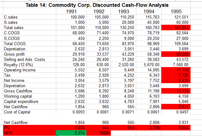
If we replace the dices by years of sales (Income statement) and use from Monte Carlo method to iterate calculations, we will reach to the rule of 50 %+. (Please see below pic)


On above spreadsheet, we have sales for year 3, 4 and 5. Then I use different probability distribution and different growth rate for CUT OFF. By one way data table, you can see an average of P (x) is equal to 53.9% by standard deviation of 0.000499.
 P (x) = P (year5 ≤ ((2*year4) – year3)) = 53.9%
It means that there is a probability more than 50% in which sales in year 5 will be less than or equal to twice sales in year 4 minus sales in year 3.
You can check this theorem (50 %+) for all income statements, annual reports and so on.
Even though we have found out this theorem, there is still more than 40 % risk to use this theorem. But, how can we decrease the risk of projection for assumptions or increase the probability prediction of our assumptions?
For deducting this risks, we have to generate other theorems by increasing the number of dices or changing the functions.

Friday, August 26, 2016

A Modified Template for Financial Section of a Business Plan

Following to article of "A Template for Financial Section of a Business Plan" posted on link: http://emfps.blogspot.com/2016/08/a-template-for-financial-section-of.htm,
the purpose of this article is to develop and improve previous template. So, I am willing to introduce you a new ratio (S) extracted from some new theorems in mathematics in which by using this ratio, we will be able to focus on only one assumption and eliminate other assumptions for our analysis. In fact, by changing other assumptions, this ratio (S) always stays the constant.   

Developing of Previous Template

In previous template, we had only one column for our assumptions. It means, by changing a variable (assumption), the changes for all years are the same. For instance, if we change the growth of sales from 4% t0 6%, the NPV shows us a growth of 6% for year 1, year 2, year 3 and so on. Please see 
below pic


In reality, there is not the same growth for all years. Therefore, I added other cells on my spreadsheet where we will have a set of assumptions for each year. This gives us the opportunity for better 
analysis by using the Monte Carlo method. Please see blow pic:


The Improve of Previous Template

In new template, I added new assumption which is the Tax rate.  In previous template, we have a big problem when EBTI is negative because we have already added tax payment to net income. In this case, there is the concept which is named NOL.
What is NOL? It is Net Operating Loss in which we can deduct our NOL from the taxes we paid in prior years and get a refund, or we can apply it to future years to lower our tax bill.
This will help us to recover some net operating losses but usually not all. 
The concept of NOL is the complicated and you cannot easily claim your NOL. Some people believe to deduct entire NOL from future taxes (Tax loss carry forwards) or to add tax payment to net income when EBTI is negative (my previous template). Let us see below example:

 Assume Company X has net sales of $2,000,000 but expenses of $2,200,000. Its net operating loss is $2,000,000 - $2,200,000 = -$200,000.
Company X will probably not have to pay taxes that year, because it has negative taxable income. But let's assume that next year, Company X makes more sales and records $700,000 of taxable income. Company X pays a corporate tax rate of 40%.
Normally, the company would need to pay $700,000 x 40% = $280,000 in taxes. But because it had a tax loss carry forward from last year, it can apply last year's loss to this year's tax bill, reducing it significantly (or even to $0, depending on the jurisdiction Company X is in).
Let's assume that Company X can apply the entire -$200,000 tax loss carryforward to this year's tax bill. Instead of owing $700,000 x 40% = $280,000 in taxes, Company X now owes only ($700,000 - $200,000) x 40% = $200,000 in taxes.

But other people say another story as follows:

"It's rare to see a company acquired for the purpose of NOLs today (at least through a direct acquisition). This is because of 382 limitations on the usability of NOLs in the case of a change in control of a company's equity rendering your NOLs almost worthless on a present value basis. NOLs are currently limited to 3.98% of the value of the company during a change of control. This number is determined by the IRS monthly and (along with the value of the company for 382 purposes) will be fixed at the time of the change of control. Based on your business and applicable tax laws, you may also have to distinguish between cash taxes and accounting taxes. The actual formula for NOI after taxes is simply: NOI - taxes. This is equivalent to (1-taxes) * NOI if your taxes are positive, but should be just NOI since your taxes are zero if your NOI is negative."

Therefore, we have the pessimistic and optimistic comments. Anyway, I choose the pessimistic situation because here is a good opportunity for our analysis as follows:

For obtaining zero taxes on my spreadsheet when NOI is negative, I use a simple trick in which I add one row under item of tax payment (Adjusted tax payment) by below formula on all months and years of cash flow statement:

=IF (B36>0; B36; 0)-B36

Please see below pics:


In this case, if your tax payment is negative, adjusted tax payment will be positive where the total sum is zero. But if your tax payment is positive, adjusted tax payment will be zero.
Then, on spreadsheet of Income statement, I add tax payment and adjusted tax payment.


But what is good opportunity?

Above trick gives us a good opportunity on our analysis. If we change the tax rate for each year but NPV, IRR and also Enterprise value do not change, it means that the combination of other assumptions presents net operating loss in its year. For example: you can see when I change tax rate in year 4 and year 5, NPV does not change. Therefore, we have net losses in year 4 and year 5. (Please see below pics)


A New Ratio (S)

Now, let me introduce you a new ratio that if you apply it on each assumption, by changing other assumptions this ratio always stay the constant.
Example:

I consider Cost of Capital as base of assumption to generate this new ratio. Of course, we can choose any assumption as the base of calculation this ratio.
- First, I use form a sensitivity analysis for the Cost of capital and NPV. (see below pic)


 - Then, the ratio of "S" is equal to NPV 3 minus NPV 2 divide NPV 4 – NPV 1

S = (NPV3 – NPV 2) / (NPV 4 – NPV 1)

We can use from IRR and also Enterprise value instead NPV.
In below pic, you can see the ratio of "S" has been calculated by using above formula for all assumptions:


Now, I change all assumptions except the Cost of Capital in below pic:


As you can see, the ratio of "S" will stay the constant for all changes of assumptions.

Indeed, what is application of the ratio of "S" for our analysis?
For answering to above question, at the first we should familiar to a new theorem of mathematics which is the rule of 0.333333….
Then we can start our analysis by using the Monte Carlo Method.
Of course, there is another ratio which is named ratio of "P". This ratio has also the property just like ratio of "S" where by changing all assumptions ratio "P" stays the constant. The formula for ratio "P" is as follows:

P = (NPV 2 – NPV1) / (NPV3 – NPV2) or
P = (EV2 – EV1) / (EV3 – EV2) or

P = (IRR2 – IRR1) / (IRR3 – IRR2)

Please see below pic:


Now, I change all assumptions and you can see ratio "S" and "P" stay the constant. Please see below pic:


Are there other ratios which have the same property?

Tuesday, August 16, 2016

The Calculation of Royalty Rate

Are you an engineer? What do you think about the value of your job? How can we get the value of engineering in a company? Or how can we calculate Intellectual property or royalty rate of a company?
To analyze some financial cases, we have to calculate the intellectual property of the company in additional to look at the book value on balance sheet.

Please see the case of "Yeats Valves and Controls Inc.". The end of first page of this case, Porter said: "YVC's prospects are brighter than ever. You have technology to die for. With our intellectual property and new products coming along, there is a lot of hidden value in this company that's not 
reflected on the balance sheet. Be a realist about the value"  

There are many papers and references to measure the intellectual property of a company. In this article, I chose a very fascinating hand book which presents six different methods to price the intellectual property of early-stage technologies.
The reference is as follows:

"ipHandbook of Best Practices"

Chapter 9.3 (2007) titled: "Pricing the Intellectual Property of Early-Stage
of Basic Valuation Technologies: A Primer Tools and Considerations" by RICHARD    RAZGAITIS

Posted on below link:


Even though I can say to you that above reference is very useful and interesting materials, there are some mistakes taken on method of Discounted Cash-Flow Analysis (method IV) and Table 14. For instance, when you read this method, you cannot still calculate the royalty rate. Your big question is: How has the royalty rate (12.6%) been calculated?

The purpose of my article is to improve and to explain the true method of Discounted Cash-Flow Analysis for calculating the royalty rate.

What should the items be improved?

1. Mistakes on calculations
2. The lack of enough information
3. The lack of good explanations

Let me start by the mistakes on calculations:

Here is Table 14:


As you can see, the calculation of all present values and total sales in 1995 are wrong. I corrected them on below spread sheet (Red highlights are true values):


2. The lack of enough information

When you start a discounted cash flow analysis, you should consider a terminal value for the end of your period. Because you have not the infinity cash in or cash out. Therefore, you should terminate and close your analysis by evaluating the value of your business in the end of the period. The formula for calculating Terminal value is as follows:

Terminal Value =
Free cash flow in the end of period * (1- terminal growth rate %) / (Cost of Capital % - terminal growth rate %)

For this analysis, I consider 2% for terminal growth rate. Please see my calculation of terminal value and also NPV on below spread sheet:


3. The lack of good explanations

The most important part of this article is, to calculate the royalty rate. The above reference do not show us how we can get the royalty rate equal to 12.6%.
Let me tell you the method as follows:

- At the first, you should eliminate amounts of Specialty product sales, Cost of specialty product sales and Royalty payment at 12.6% on your spread sheet and then calculate NPV just like below cited (Yellow highlights):


- In final step, you should add above amounts again and apply the sensitivity analysis for the royal rate and NPV in which NPV in both step are the same, it shows you percentage of the royalty rate as follows:


As you can see, the royalty rate is not 12.6% but it is equal to 55%.

Monday, August 1, 2016

A Template for Financial Section of a Business Plan Plus Monte Carlo Analysis

The most important part of a business plan is to prepare the financial section and the most crucial part of the financial section is, to predict assumptions because you should prove that your business plan is feasible or not.
The purpose of this article is to make a template of financial section on excel spreadsheets in which all excel files are connected together and also assumptions. In this case, you will be able to track 
rapidly your analysis by changing the assumptions.

Good news is to apply Monte Carlo analysis on this template in which you can control the risks of the assumptions and see the impact of them on your performance by using the method mentioned in below article: 


"Discounted Cash Flow Analysis plus Monte Carlo Method to Analyze Share Price of a Company" 
A sample for financial section of a business plan in service industry has been practiced on this 
template.

Financial Section of a Business Plan

A financial section of business plan is started by the assumptions. You can always change your assumptions and show to your client that this business plan is feasible or vice versa. Therefore, the assumptions play the most important role in your business plan. Traditionally, the people forecast the assumptions derived from financial data previous years of company or economic indicators. Definitely this method is not true due to high speed changes in the world. We have not still an accurate method to find out true assumptions. In fact, if we had a precise model to guess the assumptions, we could anticipate some share prices or the performances in stock markets. As I stated in my article of "External Real Forces and Pseudo-Forces to Design a Strategic Plan: Fuzzy logic Vs. Classic Logic" posted on link: http://emfps.blogspot.com/2013/12/external-real-forces-and-pseudo-forces.html, maybe the mathematics will give us an optimized model to forecast the 
assumptions in the near future.

What are the assumptions? They can be as follows:

- Initial investment
- The growth rate of the sales per year
-The growth rate of variable costs per year (COGS)
- The growth rate of fixed costs per year
- Terminal value growth rate
- The cost of capital (discounted rate) in each year
- Taxes
-Interest rates

When we obtain the assumptions, we should develop a cash flow statement for 12 months per year and predict it for 3 or 5 years in accordance with our initial investment and costs budgeting and also our assumptions. This is the statement that shows the money how is moving in and out of our business. Making a cash flow statement is very important for our business plan because it is the basic of profit – loss projection, balance sheet and finally our analysis.
After developing a cash flow statement, we will be able to prepare an Income statement projection (3 or 5 years) and by using data generated in profit – loss statement, we can make the Balance sheet projection for 3 or 5 years.
When we finish to create the cash flow statement, Income statement and Balance sheet, we will be ready to go our analytic process included in below steps:

- To calculate Key Ratios (Viability analysis) by using of Income statement and Balance sheet
- Break – Even Analysis by using of the Sales, Variable costs and Fixed costs
- Discounted Cash Flow Analysis
In my opinion, the most important part of our analytic process is, to go to the discounted cash flow analysis which is included three below steps:
- Pay Back analysis
- IRR analysis
- NPV analysis

Finally, we will have six excel files connected together and our assumptions as financial section of 
our business plan as follows:

- Cash flow statement
- Income statement
- Balance sheet
- Key Ratios (Viability analysis)
- Break – Even Analysis
- Discounted Cash Flow Analysis


A Sample of Financial Section for Business Plan in Service Industry

I have made a sample of a financial section for a business plan in the tourism industry. You can practice and also utilize this sample for commercial purposes. This sample can be used for many service industries, such as food service, boarding houses, restaurants, transportation, and so on
Firstly, we have assumptions as follows:


Then we develop a cash flow statement:


After that, we prepare an Income statement projection:


According to above mentioned, we can make Balance sheet:


Now, we can start the discount cash flow analysis as follows:


Then, we use from Pay back method:


Next analysis is, IRR and NPV method:


In this case, if we change some variables of our assumptions, we can see that all discounted cash flow analysis simultaneously change so that our business plan will not be feasible:


In fact, this is a goal for our analysis. In the near future, I will show you, how we can use from this method to reach the optimized variables? For instance, how can we obtain the bottom line for unit price of the goods?
Finally, we have Key ratios and Break – Even Analysis as follows: